Root mean square values
The reason for using what seems a rather
complicated definition is as follows. The power P used in a resistor R is proportional to the
square of the current:
P = I2R
But with alternating current the value of I and
therefore of P changes, and so:
mean value of P = (mean value of i2) x R = I2R = (mean value of V2)/R where
V = √(mean value of V2) = root mean square (r.m.s) volage
We can therefore define the
r.m.s. value as that voltage that would dissipate power at the same rate as a d.c. current of the
same value.
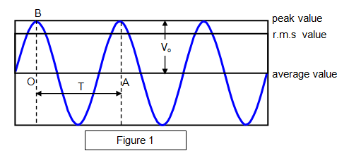
The relation between the peak and r.m.s. values for a sinusoidal wave can be seen in Figure 1. It can be shown that
the r.m.s. value of voltage V is related to the peak value V
o by the equation:
Root mean square voltage: V = Vo/√2 = 0.707Vo)
Similarly, for the current we have:
Root mean square current: I = Io/2√2 = 0.707Io)
In Britain the voltage supply is 230 V; this is the r.m.s. value, and so the peak value is 230/0.707 or in the region of 325
V.
Proof of the value of the r.m.s. current
Let the current vary with time in the following way:
i= I
osin(
w)t
where ω is a constant related to the frequency f by
the equation
w = 2
pf.
By definition the r.m.s. current (I) is
I = (mean value of
i
2)
1/2 = (mean value of sin
2(ωt))
1/2But sin
2(
wt) = ˝ – ˝ cos (2ωt), and the
mean value of cos (2ωt) is 0.
Therefore the mean value of sin
2 (ωt) = ˝ , and therefore I = I
o(˝)
1/2 =
I
o/(2)
1/2
It is
important to realise that the general definition of r.m.s. value applies to any type of
varying signal and not simply to one that varies sinusoidally. For example, it is quite
possible for a square wave to have an r.m.s. value. The specific equation above
however applies to sinusoidal variations only.
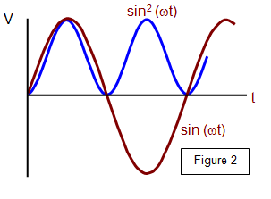
The variation of both sin(ωt) and sin2(ωt) are shown in Figure
2.
A VERSION IN WORD IS AVAILABLE ON THE SCHOOLPHYSICS USB