Uncertainties and errors in graphs

The uncertainty in a measurement can be shown on a graph as an error bar. This bar is drawn above and below the point (or from side to side) and shows the uncertainty in that measurement.

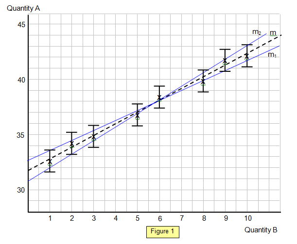
In the example shown below (Figure 1) we will assume that only quantity A has an uncertainty and that this is +/- 1. For example the reading of A for B = 6 is given as 38.4 but because of the uncertainty actually lies somewhere between 37.4 and 39.4.

The line of gradient m is the best-fit line to the points where the two extremes m₁ and m₂ show the maximum and minimum possible gradients that still lie through the error bars of all the points.


In the example m₁ = [43.2-30.8]/10 = 1.24 and m₂ = [41.7-32.7]/10 = 0.90.

The slope of the best fit line (m) = [42.4-31.8]/10 = 1.06

In the example the uncertainty is [1.24-0.90]/1.06 = 32%

Alternatively the value of the gradient can be written as 1.06 +/-0.17



If the lines are used to measure an intercept (in this case on the Y (quantity A) axis) then there will be an uncertainty in this value also.

For the line of gradient m the intercept is 31.8
For the line of gradient m₁ it is 30.8 and for the line of gradient m₂ it is 32.7.

So the value for the intercept could be quoted as 31.8 +/-1.0.

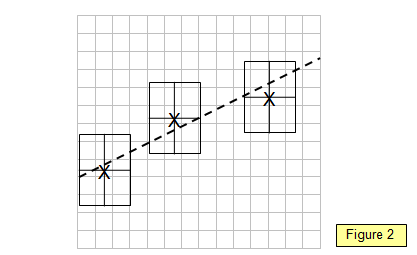
If there is an uncertainty in both the quantities A and B then instead of an error bar you would have an error rectangle. The maximum and minimum gradient lines should pass through the error rectangle for each point on the graph (see Figure 2).



N.B the comments in this section about uncertainty and errors apply to a curve as well as a straight line graph although of course the gradient of the graph would vary along the curve.